Introduction
A thermocouple operates on the thermoelectric effect between two dissimilar conductors, converting a temperature difference into a small electrical voltage. In practice, a thermocouple thermometer does not measure temperature directly. It first measures a signal typically in the microvolt or millivolt range.
One important point is that thermocouple output voltage is not perfectly linear with temperature. For example, an identical temperature increase of 100 °C does not necessarily produce exactly the same voltage change at different parts of the measurement range. The degree of nonlinearity also varies between thermocouple types.
For this reason, a thermocouple thermometer cannot simply multiply the measured voltage by one fixed conversion factor. It must perform linearization using the standardized thermoelectric voltage–temperature relationship for the selected thermocouple type.
Modern digital thermocouple thermometers typically integrate signal conditioning, analog-to-digital conversion, cold junction compensation, and linearization into the instrument so that the user sees the final temperature directly.
Key Points
● Thermocouple voltage has a nonlinear relationship with temperature and therefore requires linearization;
● Different thermocouple types, such as K, J, T, and E, require their own voltage–temperature characteristics;
● A thermocouple thermometer normally performs cold junction compensation before converting the equivalent thermoelectric voltage into temperature;
● Common linearization methods include lookup tables, interpolation, polynomial calculation, and piecewise linearization;
● Linearization is only one part of the measurement chain. ADC performance, analog circuitry, the cold junction sensor, and the thermocouple itself also affect overall measurement accuracy.
Why Do Thermocouples Require Linearization?
If thermocouple output voltage were perfectly proportional to temperature, the conversion could be represented by a simple linear equation:
$$
T=aE+b
$$
where T is temperature, E is thermocouple voltage, and a and b are fixed coefficients.
Real thermocouples, however, do not behave in this ideal way.
The thermoelectric sensitivity of a thermocouple can be described by its Seebeck coefficient, and this coefficient changes with temperature. Over a wide temperature range, the voltage–temperature characteristic therefore forms a curved nonlinear relationship rather than a straight line.
This means:
● The voltage change produced by a 1 °C temperature increase at one temperature may differ from the change produced at another temperature;
● Different thermocouple types use different metal or alloy combinations and therefore have different nonlinear characteristics;
● The wider the temperature range, the greater the potential error when a single fixed linear coefficient is used.
For accurate or wide-range measurements, the thermometer must compensate for this nonlinearity using the standardized characteristic of the relevant thermocouple type. This process is referred to as linearization.
What Does a Thermocouple Thermometer Actually Measure?
The measurement input of a thermocouple thermometer is thermoelectric voltage, not temperature itself.
Thermocouple signals are typically very small. Common base-metal thermocouples usually generate voltages from the microvolt range up to several tens of millivolts across their operating range. The instrument therefore normally performs the following steps:
● The thermocouple probe generates a thermoelectric voltage;
● The analog front end conditions and, where necessary, amplifies the low-level signal;
● The ADC converts the analog signal into digital data;
● The instrument measures the cold junction temperature near the thermocouple terminals;
● Cold junction compensation is applied;
● The compensated voltage is linearized according to the selected thermocouple type;
● The calculated value is displayed in °C, °F, or another configured temperature unit.
The temperature shown on a digital thermocouple thermometer is therefore the result of several measurement and calculation stages.
Why Must Linearization Match the Thermocouple Type?
Different thermocouple types use different conductor combinations, resulting in different voltage–temperature characteristics.
For example:
● Type K thermocouples typically use nickel-chromium and nickel-based alloy conductors;
● Type J thermocouples typically use iron and copper-nickel alloy;
● Type T thermocouples typically use copper and copper-nickel alloy;
● Type E thermocouples typically use nickel-chromium and copper-nickel alloy.
Because each material combination produces a different thermoelectric voltage, two different thermocouple types exposed to the same temperature may generate different millivolt values.
The thermometer must therefore know which thermocouple type is connected.
If the instrument calculates temperature using a Type K characteristic while a Type J thermocouple is actually connected, the measured voltage may be correct but the displayed temperature can still be significantly wrong.
Multi-input or multi-type thermocouple thermometers therefore require the user or system configuration to select the correct K, J, T, E, or other thermocouple type.
What Is the Relationship Between Linearization and Cold Junction Compensation?
A thermocouple responds to the temperature difference between its measuring junction and reference junction rather than directly measuring an absolute temperature.
Standard thermocouple reference tables are generally defined relative to a reference junction at 0 °C. In an actual thermometer, however, the input terminals may be at 20 °C, 25 °C, or another ambient temperature. The measured voltage therefore cannot normally be converted directly using the standard reference table.
This is why thermocouple thermometers require cold junction compensation (CJC).
A typical digital calculation can be expressed as:
$$
E_{total}=E_{measured}+E_{CJC}
$$
where:
● (E_{measured}) is the thermocouple voltage measured by the instrument;
● (E_{CJC}) is the equivalent thermoelectric voltage corresponding to the measured cold junction temperature for the selected thermocouple type;
● (E_{total}) is the equivalent thermoelectric voltage referenced to the standard reference condition.
The instrument then calculates:
$$
T=f^{-1}(E_{total})
$$
to obtain the measuring-junction temperature.
Cold junction compensation is therefore not simply a matter of adding the cold junction temperature directly to a temperature difference. The calculation must follow the thermoelectric characteristic of the selected thermocouple.
In a complete measurement system, cold junction compensation corrects the reference-junction condition, while linearization corrects the nonlinear voltage–temperature relationship. They perform different functions but both are essential to accurate temperature conversion.
How Does Lookup-Table Linearization Work?
Standardized thermocouple characteristics can be represented by voltage–temperature tables. For a selected thermocouple type, the system can use the compensated thermoelectric voltage to determine the corresponding temperature.
In practice, a digital thermometer does not necessarily store every possible temperature point. It may store representative data points and interpolate between them.
If the measured voltage satisfies:
$$
E_1<E<E_2
$$
and the corresponding temperatures are (T_1) and (T_2), linear interpolation over a sufficiently small interval can be expressed as:
$$
T=T_1+\frac{E-E_1}{E_2-E_1}(T_2-T_1)
$$
Although the complete thermocouple characteristic is nonlinear, it can be approximated accurately by a straight line over a sufficiently narrow segment.
Lookup-table and interpolation methods are intuitive, stable, and widely used in digital measurement systems.
How Is Polynomial Linearization Performed?
Another method is to approximate the standardized thermocouple characteristic using a polynomial equation.
A typical form is:
$$
T=a_0+a_1E+a_2E^2+a_3E^3+\cdots+a_nE^n
$$
where:
● T is the calculated temperature;
● E is the compensated thermoelectric voltage;
● (a_0, a_1, a_2 \ldots a_n) are coefficients applicable to the selected thermocouple type and range.
The processor substitutes the measured thermoelectric voltage into the relevant equation and calculates the temperature.
A single coefficient set is not necessarily used across the entire thermocouple range. To maintain high accuracy, different polynomial coefficients may be specified for different temperature or voltage intervals.
Polynomial linearization therefore requires correct identification of:
● Thermocouple type;
● Current thermoelectric voltage range;
● Coefficient set applicable to that range;
● Valid range of the equation.
Using a polynomial outside its specified range can significantly increase conversion error.
What Is Piecewise Linearization?
Piecewise linearization divides the entire nonlinear thermocouple characteristic into a number of smaller sections and approximates each section as a straight line.
For example:
● Range A uses one slope and intercept;
● Range B uses another set of parameters;
● Range C uses another set again.
Because each individual segment is relatively narrow, the local characteristic is closer to linear. This method can provide a practical balance between computational complexity and conversion accuracy.
Piecewise linearization is conceptually similar to lookup-table interpolation, although the implementation method may differ.
Modern microcontrollers generally provide sufficient processing power and memory to use lookup tables, interpolation, polynomials, piecewise methods, or combinations of these techniques.
Typical Thermocouple Linearization Process
A typical digital thermocouple thermometer follows this general sequence:
● The measuring junction is brought into adequate thermal contact with the target;
● The thermocouple generates a voltage related to the temperature difference between the measuring and reference junctions;
● The analog front end acquires and conditions the low-level signal;
● The ADC converts the analog voltage into digital data;
● The thermometer measures the cold junction temperature near the input terminals;
● The equivalent cold-junction thermoelectric voltage is calculated for the selected thermocouple type;
● The measured voltage and cold-junction equivalent voltage are combined;
● The compensated voltage is converted using the corresponding standardized thermocouple characteristic;
● The measuring-junction temperature is obtained;
● The value is displayed in °C or °F according to the instrument settings.
Linearization is therefore an important stage, but it is only one element of the complete thermocouple measurement chain.
Does Linearization Determine the Entire Accuracy of a Thermocouple Thermometer?
No.
Even if the linearization algorithm is extremely accurate, other error sources remain in the measurement system.
These include:
● Tolerance of the thermocouple probe itself;
● Material inhomogeneity and thermocouple aging;
● Incorrect use of extension or compensating cable;
● Parasitic thermoelectric voltages at connections;
● Offset and gain errors in the analog front end;
● ADC resolution, linearity, and reference-voltage errors;
● Accuracy of the cold junction temperature sensor;
● Cold junction errors caused by temperature gradients inside the instrument;
● Electromagnetic and common-mode interference;
● Errors caused by probe installation, insertion depth, and heat conduction.
Linearization error must therefore not be confused with total thermocouple thermometer error.
A high-quality thermocouple thermometer requires coordinated control of sensor performance, analog circuitry, ADC performance, cold junction compensation, digital algorithms, and thermal design.
Does a More Accurate Linearization Algorithm Always Mean More Accurate Temperature Measurement?
Not necessarily.
For example, a linearization algorithm may have a calculation error below 0.1 °C, while the connected thermocouple probe may have an allowable error of several degrees Celsius. In that case, further improving the numerical precision of the algorithm may have little effect on overall measurement accuracy.
Similarly, if the cold junction sensor is not at the same effective temperature as the thermocouple input terminals, significant error may remain even when a highly accurate standardized polynomial is used.
Thermocouple thermometer design should therefore focus on the overall measurement uncertainty, rather than maximizing the numerical precision of only one processing stage.
Why Can a Fixed μV/°C Coefficient Not Be Used Across the Entire Range?
Over a narrow temperature range, a thermocouple characteristic can often be approximated as linear, and a nominal sensitivity expressed in μV/°C may be useful for estimation.
However, thermocouple sensitivity is not constant across the complete operating range.
If a sensitivity value valid around one reference temperature is applied across the entire range, the conversion error generally increases as the temperature moves further away from that region.
Therefore:
● A local linear approximation may be suitable for narrow-range, low-accuracy estimates;
● Wide-range or precision measurements should use the standardized thermocouple characteristic.
Professional digital thermocouple thermometers generally use the latter approach.
What Is the Role of Standard Thermocouple Data in Linearization?
Industry standards define nominal voltage–temperature characteristics for each standardized thermocouple type so that thermocouples and measuring instruments from different manufacturers can use a consistent reference relationship.
These standardized characteristics may be expressed as:
● Thermoelectric voltage–temperature tables;
● Polynomial equations;
● Standard reference functions.
The software or firmware inside a thermocouple thermometer uses these relationships to convert measured voltage into temperature.
When a multi-type thermometer switches between K, J, T, E, and other thermocouple types, it is therefore not merely changing the type indicator on the display. The instrument also changes the cold-junction compensation and linearization parameters used in the calculation.
What Should Be Considered When Implementing Linearization?
● The selected thermocouple type must match the actual connected probe;
● Reference tables or polynomial coefficients for different thermocouple types must not be mixed;
● Polynomial equations must be used only within their specified valid ranges;
● Large-range extrapolation beyond standardized data should be avoided;
● Cold junction compensation should be handled correctly before final temperature conversion;
● The ADC must provide sufficient resolution and low-noise performance;
● The number of displayed decimal places does not represent the total measurement accuracy;
● Probe tolerance, wiring, cold junction compensation, electronics, and installation conditions must all be considered.
FAQ
Is a thermocouple a linear temperature sensor?
Not in the strict sense. The thermoelectric voltage generated by a thermocouple has a defined but nonlinear relationship with temperature, so digital thermometers normally apply linearization.
Why can a thermocouple thermometer not simply divide voltage by sensitivity to obtain temperature?
Because thermocouple sensitivity in μV/°C changes with temperature. A fixed sensitivity can only approximate behavior over a limited range and cannot provide accurate conversion across the complete operating range.
Can different thermocouple types use the same linearization algorithm?
The general algorithm structure may be similar, but each thermocouple type requires its own reference data or polynomial coefficients. Types K, J, T, E, and others cannot use the same conversion parameters.
Are cold junction compensation and linearization the same thing?
No. Cold junction compensation corrects for the fact that the reference junction is not at 0 °C, while linearization corrects the nonlinear relationship between thermoelectric voltage and temperature. Both are normally required for the final calculation.
Which is more accurate: lookup-table or polynomial linearization?
Accuracy cannot be determined by the method name alone. Both can provide very high conversion accuracy when the reference data, interval spacing, interpolation method, and numerical implementation are designed correctly. The choice depends mainly on processor capability, memory, and system requirements.
If a thermometer displays 0.1 °C, does that mean its accuracy is ±0.1 °C?
No. A 0.1 °C indication usually represents display resolution. Total accuracy also depends on the thermocouple probe, cold junction compensation, analog circuitry, ADC, linearization, and other error sources.
Can temperature still be calculated outside the specified linearization range?
Extrapolation beyond the specified range of standardized equations or tables is generally not recommended. Conversion error and thermocouple material stability may no longer be guaranteed. Instruments therefore often indicate an over-range condition or restrict the displayed value.
Conclusion
A thermocouple thermometer does not directly measure temperature. It first measures the small thermoelectric voltage generated by the thermocouple and then applies signal conditioning, cold junction compensation, and linearization to convert that voltage into temperature.
Because each thermocouple type has its own nonlinear voltage–temperature characteristic, a fixed μV/°C conversion factor is not suitable across a wide measurement range. Modern digital thermocouple thermometers therefore commonly use standardized lookup tables, interpolation, polynomial equations, piecewise linearization, or combinations of these methods.
Linearization is only one part of achieving accurate thermocouple measurement. Probe accuracy, cold junction compensation, analog circuitry, ADC performance, wiring, and installation conditions also affect the final result. Reliable temperature measurement therefore depends on controlling the complete measurement chain rather than only the numerical conversion algorithm.